Posts Tagged ‘Bayesian statistics’
Bayesian stuff, encore, encore, probably

So I was listening to one of my science podcasts in my usual distracted way, when a segment came on about Bayesian inference, or reasoning, or logic, woteva, and I know I’ve written about this before, but I also know that if someone asked me to explain it, I’d be lost, caught out, shamed and disgraced. Me, an inner-lechal? Come now.
So, once more into the breach – and I’m not even going to look at anything I’ve written on the topic before, nor am I going to avoid the issue by going on about the Reverend Thomas Bayes’ relatively obscure 18th century life in Tunbridge Wells, where he… oh, sorry.
Bayes’ Theorem, or Rule, says that the probability of A, given B, is the probability of B given A, times the probability of A, all divided by the probability of B. Mathematically it looks like this:
P(A|B) = P(B|A).P|(A)/P(B), – which simplifies to
P(A|B) = P(A + B)/P(B)
It’s about statistical inference apparently, and also, to some degree, about common sense and everyday experience. One tutorial puts it this way. Someone tells you, very briefly, that a friend of hers has just been diagnosed with breast cancer. You’ve just recently learned that males too can develop breast cancer. You wonder if that friend is male. What are the chances?
So the probability of maleness, given breast cancer, is equal to the probability of having breast cancer, given maleness, multiplied by the probability of being male, all divided by the probability of having breast cancer. Now, the probability of breast cancer given maleness is about one in a thousand, according to the tutorial (i.e 0.001) And the probability of being male is about one in two, or 50% (0.5), while the overall probability of getting breast cancer is 0.063 (63 in a thousand). So, putting those stats together and doing the maths results in a tiny .79% likelihood of the friend being male, assuming the stats are reliable, and there aren’t any other confounding factors. That’s well under 1%, I have to remind myself. Then again, a more efficient way to find out, as the tutorial points out, is to just ask!
So what’s a more effective scenario for using Bayesian probability? Well…
The ratio of probability of a piece of ‘information’ being true under one hypothesis, compared to it being false, is called a Bayes factor, apparently – representing ‘the amount of information we’ve learned, re our hypothesis, from the available data’. This learning is used, or can be used, to update our prior belief or understanding, to a posterior one. The whole process is one of hypothesis testing, and the belief-changing that should be attendant upon that testing. As if…
So therein lies the problem, that we don’t subject our beliefs to hypothesis-testing, at least not often, and not very much at all when we live in a community that shares those beliefs. If the Reverend Bayes lived in 21st century Adelaide, he might not be so reverential about the putative father-and-son beings he was so reverential about, presumably, in 18th century Tunbridge Wells. But how can you subject your belief in a single, omniscient, ominipotent creator god to hypothesis-testing? That’s when the concept of evidence comes in, and not just evidence about beliefs. So it seems to me that Bayesian probability has rather limited applications.
And yet, it’s pretty obvious that Bayesian woteva – reasoning, inference, probability, priors, theorems etc – has been flavour of the month for months and months and months now (and isn’t ‘month’ a funny word, come to think of it? but I digress…), though there is push-back, and even something of a turf war, between Bayesian and frequentist-type reasoning, and there are articles and videos galore about all this stuff – and I’ve been around for sixty-odd years without giving any of it the slightest thought. Here’s a quick summary from somewhere:
the frequentist approach assigns probabilities to data, not to hypotheses, whereas the Bayesian approach assigns probabilities to hypotheses. Furthermore, Bayesian models incorporate prior knowledge into the analysis, updating hypotheses probabilities as more data become available.
As one nice video puts it, using a coin flip, for those who see the coin land, the datum shows that the coin shows heads, say, and this isn’t probable, it’s a fact. For those who don’t, there’s a 50% probability that the coin will show heads. The Bayesian bases her conjecture on her prior knowledge that coins have two sides, but if she learns that the coin-flipper is a trickster with a double-headed coin (thus updating her prior knowledge) she updates the hypothesis based on this datum. So it just seems to be a difference between data and knowledge of data. I’m not quite sure I understand what all the fuss is about. And yet… As Steven Pinker points out, in his book Rationality:
In recent decades Bayesian thinking has skyrocketed in prominence in every scientific field. Though few laypeople can name or explain it, they have felt its influence in the trendy term ‘priors’, which refers to one of the variables in the theorem.
I haven’t myself noted the trendiness of priors but I’ve never really been in academia. In any case the term seems pretty basic, and I’m just not sure about the need to ‘mathematise’ it all. Pinker himself first describes Bayes’ Rule in verbal/arithmetical terms – posterior probability = prior probability x likelihood of the data/commonness of the data – which he then translates into English, and after that into common sense, i.e ‘now that you’ve seen the evidence, how much should you believe the idea?’ So, if you’re an evidence-conscious type, you should generally be fine, methinks. I have heard it said, though, that many people even at high levels of academia trip themselves up because they ‘forget’ to apply Bayes’ Rule. I suspect, though, that it’s not so much forgetting as motivated reasoning or ‘my side bias’, generally a tougher nut to crack…
References
You know I’m all about that Bayes: crash course stats (video)
Are you Bayesian or Frequentist? video, Cassie Kozyrkov
Steven Pinker, Rationality, 2021
https://johnhorgan.org/cross-check/bayes-theorem-and-bullshit
Bayesian probability, sans maths (mostly)

Okay time to get back to sciency stuff, to try to get my head around things I should know more about. Bayesian statistics and probability have been brought to the periphery of my attention many times over the years, but my current slow reading of Daniel Kahneman’s Thinking fast and slow has challenged me to master it once and for all (and then doubtless to forget about it forevermore).
I’ve started a couple of pieces on this topic in the past week or so, and abandoned them along with all hope of making sense of what is no doubt a doddle for the cognoscenti, so I clearly need to keep it simple for my own sake. The reason I’m interested is because critics and analysts of both scientific research and political policy-making often complain that Bayesian reasoning is insufficiently utilised, to the detriment of such activities. I can’t pretend that I’ll be able to help out though!
So Thomas Bayes was an 18th century English statistician who left a theorem behind in his unpublished papers, apparently underestimating its significance. The person most responsible for utilising and popularising Bayes’ work was the French polymath Pierre-Simon Laplace. The theorem, or rule, is captured mathematically thusly:
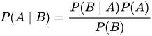
where A and B are events, and P(B), that is, the probability of event B, is not equal to zero. In statistics, the probability of an event’s occurrence ranges from 0 to 1 – meaning zero probability to total certainty.
I do, at least, understand the above equation, which, wordwise, means that the probability of A occurring, given that B has occurred, is equal to the probability of B occurring, given that A has occurred, multiplied by the probability of A’s occurrence, all divided by the probability of B’s occurrence. However, after tackling a few video mini-lectures on the topic I’ve decided to give up and focus on Kahneman’s largely non-mathematical treatment with regard to decision-making. The theorem, or rule, presents, as Kahneman puts it, ‘the logic of how people should change their mind in the light of evidence’. Here’s how Kahneman first describes it:
Bayes’ rule specifies how prior beliefs… should be combined with the diagnosticity of the evidence, the degree to which it favours the hypothesis over the alternative.
D Kahneman, Thinking fast and slow, p154
In the most simple example – if you believe that there’s a 65% chance of rain tomorrow, you really need to believe that there’s a 35% chance of no rain tomorrow, rather than any alternative figure. That seems logical enough, but take this example re US Presidential elections:
… if you believe there’s a 30% chance that candidate x will be elected President, and an 80% chance that he’ll be re-elected if he wins first time, then you must believe that the chances that he will be elected twice in a row are 24%.
This is also logical, but not obvious to a surprisingly large percentage of people. What appears to ‘throw’ people is a story, a causal narrative. They imagine a candidate winning, somewhat against the odds, then proving her worth in office and winning easily next time round – this story deceives them into defying logic and imagining that the chance of her winning twice in a row is greater than that of winning first time around – which is a logical impossibility. Kahneman places this kind of irrationalism within the frame of system 1 v system 2 thinking – roughly equivalent to intuition v concentrated reasoning. His solution to the problem of this kind of suasion-by-story is to step back and take greater stock of the ‘diagnosticity’ of what you already know, or what you have predicted, and how it affects any further related predictions. We’re apparently very bad at this.
There are many examples throughout the book of failure to reason effectively from information about base rates, often described as ‘base-rate neglect’. A base rate is a statistical fact which should be taken into account when considering a further probability. For example, when given information about the character of a a fictional person T, information that was deliberately designed to suggest he was stereotypical of a librarian, research participants gave the person a much higher probability of being a librarian rather than a farmer, even though they knew, or should have known, that the number of persons employed as farmers was higher by a large factor than those employed as librarians (the base rate of librarians in the workforce). Of course the degree to which the base rate was made salient to participants affected their predictions.
Here’s a delicious example of the application, or failure to apply, Bayes’ rule:
A cab was involved in a hit-and-run at night. Two cab companies, Green Cabs and Blue Cabs, operate in the city. You’re given the following data:
– 85% of the cabs in the city are Green, 15% are Blue.
– A witness identified the cab as Blue. The court tested the reliability of the witness under the circumstances that existed on the night of the accident and concluded that the witness correctly identified each one of the two colours 80% of the time and failed 20% of the time.
What is the probability that the car involved in the accident was Blue rather than Green?
D Kahneman, Thinking fast and slow, p166
It’s an artificial scenario, granted, but if we accept the accuracy of those probabilities, we can say this: given that the base rate of Blue cars is 15%, and the probability of the witness identifying the car accurately is 80%, we have this figure for the dividend – (.15/.85) x (.8/.2) =.706. Dividing this by the range of probabilities plus the dividend (1.706) gives approximately 41%.
So how close were the research participants to this figure? Most participants ignored the statistical data – the base rates – and gave the figure of 80%. They were more convinced by the witness. However, when the problem was framed differently, by providing causal rather than statistical data, participants’ guesses were more accurate. Here’s the alternative presentation of the scenario:
You’re given the following data:
– the two companies operate the same number of cabs, but Green cabs are involved in 85% of accidents
– the information about the witness is the same as previously presented
The mathematical result is the same, but this time the guesses were much closer to the correct figure. The difference lay in the framing. Green cabs cause accidents. That was the fact that jumped out, whereas in the first scenario, the fact that most clearly jumped out was that the witness identified the offending car as Blue. The statistical data in scenario 1 was largely ignored. In the second scenario, the witness’s identification of the Blue car moderated the tendency to blame the Green cars, whereas in scenario 1 there was no ‘story’ about Green cars causing accidents and the blame shifted almost entirely to the Blue cars, based on the witness’s story. Kahneman named his chapter about this tendency ‘Causes trump statistics’.
So there are causal and statistical base rates, and the lesson is that in much of our intuitive understanding of probability, we simply pay far more attention to causal base rates, largely to our detriment. Also, our causal inferences tend to be stereotyped, so that only if we are faced with surprising causal rates, in particular cases and not presented statistically, are we liable to adjust our probabilistic assessments. Kahneman presents some striking illustrations of this in the research literature. Causal information creates bias in other areas of behaviour assessment too, of course, as in the phenomenon of regression to the mean, but that’s for another day, perhaps.